FCDD: Fully Convolutional Data Description
1. Background
1.1 Deep One-Class Classification.
It performs anomaly detection by learing a neural network to map nomial samples near a center \(\textbf{c}\) in output space, causing anomalies to be mapped away. Hypersphere Classifier (HSC) is used for semi-supervised one-class classification like DSVDD (Ruff et al., 2018).
HSC objective function :
$$ \min_{\mathcal{W}, \textbf{c}} \frac{1}{n}\sum^{n}_{i=1}(1-y_i)h(\phi(X_i;\mathcal{W})-\textbf{c}) - y_{i}\log(1-\exp(-h(\phi(X_{i};\mathcal{W})-\textbf{c})))$$
Here, \(h\) is the pseudo-Huber loss, \(h(\textbf{a}) = \sqrt{\|\textbf{a}\|^{2}_{2}+1}-1\), which is a robust loss that interpolates from quadratic to linear pernalization. The HSC encourages \(\phi\) to map nomial samples near \(\textbf{c}\) and anomalous samples away from the center \(\textbf{c}\) (the center \(\textbf{c}\) corresponds to the bias term).
1.2 Fully Convolutional Architecture.

Fully convolutional network (FPN) maps an image to a matrix of features, i.e. \(\phi : \mathbb{R}^{c\times h\times w} \rightarrow \mathbb{R}^{1\times u\times v}\) by using alternating convolutional and pooling layers only, and does not contain any fully connected layers. A core property of a convolutional layer is that each pixel of its output only depends on a small region of its input, known as the output pixel’s receptive field. The outcome of several stacked convolutions also has receptive fields of limited size and consistent relative position, though their size grows with the amount of layers. Because of this an FCN preserves spatial information.
2. Methodology
2.1 Fully Convolutional Data Description (FCDD).
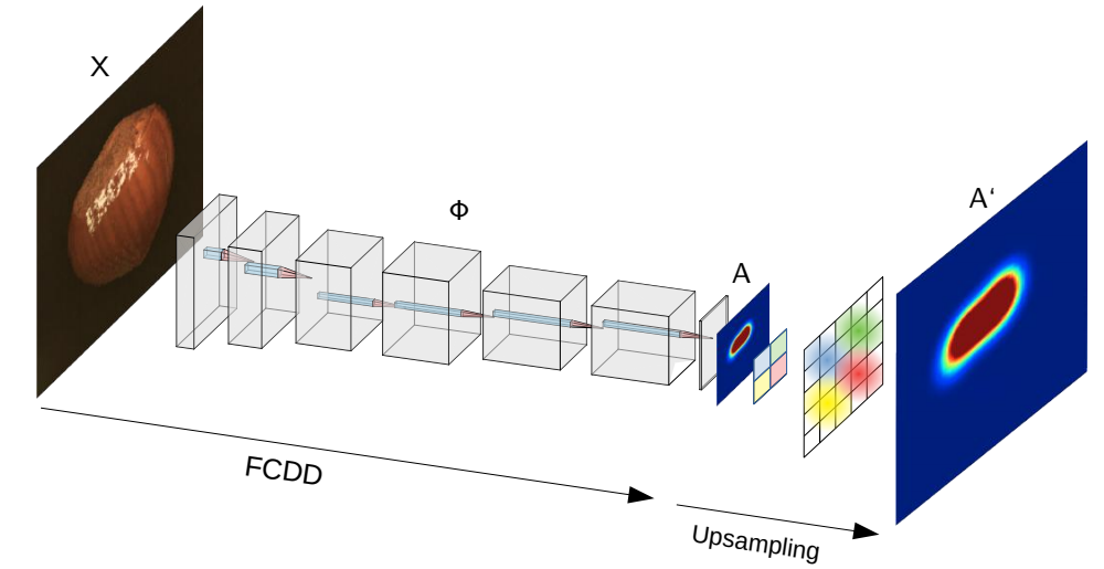
By taking advantage of FCNs along with the HSC above, output features of FCCD preserve spatial information and also serve as a downsampled anomaly heatmap. FCDD is trained using samples that are labeled as nominal or anomalous. Anomalous samples can simply be a collection of random images which are not from the nominal collection. The use of such an auxiliary corpus has been recommended in recent works on deep AD, where it is termed Outlier Exposure (OE). Furthermore, in the absence of any sort of known anomalies, one can generate synthetic anomalies, which we find is also very effective (unsupervised learning).
With an FCN \(\phi : \mathbb{R}^{c\times h\times w} \rightarrow \mathbb{R}^{1\times u\times v}\) the FCDD object utilizes a pseudo-Huber loss on the FCN output matrix \(A(X) = (\sqrt{\phi(X;\mathcal{W}+1)^{2}}-1)\), where all operations are applied element-wise.
FCDD objective function :
$$ \min_{\mathcal{W}} \frac{1}{n}\sum^{n}_{i=1}(1-y_i)\frac{1}{u\cdot v}\|A(X_{i})\|_{1} - y_{i}\log(1-\exp(-\frac{1}{u\cdot v}\|A(X_{i})\|_{1}))$$
The objective maximizes \(|A(X)\|_{1}\) for anomalies and minimizes it for nominal samples, thus we use \(|A(X)\|_{1}\) as the anomaly score. The shape of these regions depends on the receptive field of the FCN. Note that \(A(X)\) has spatial dimensions \(u \times v\) and is smaller than the original image dimensions \(h \times w\).
2.2 Heatmap Upsampling.
Because we generally lack ground-truth anomaly maps in an AD setting during training, it is not possible to train an FCN in a supervised way to upsample the low-resolution heatmap \(A(X)\). For this reason, an upsampling scheme based on the properties of receptive fields is needed.
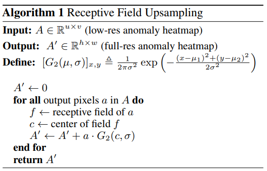
For every output pixel in \(A(X)\) there is a unique input pixel which lies at the center of its receptive field. It has been observed before that the effect of the receptive field for an output pixel decays in a Gaussian manner as one moves away from the center of the receptive field. So, \(A(X)\) is upsampled by using a strided transposed convolution with a fixed Gaussian kernel. The kernel size is set to the receptive field range of FCDD and the stride to the cumulative stride of FCDD.
3. Experiments
3.1 Standard Anomaly Detection BenchMarks
The common AD benchmark is to utilize these classification datasets in a one-vs-rest setup where the “one” class is used as the nominal class and the rest of the classes are used as anomalies at test time. For training, only nominal samples is used as well as random samples from some auxiliary Outlier Exposure (OE).
Fashion-MNIST. Fashion-MNIST using EMNIST or grayscaled CIFAR-100 as Outlier Exposure (OE). Network that consists of three convolutional layers with batch normalization, separated by two downsampling pooling layers is used.
CIFAR-10. As OE CIFAR-100 is used, which does not share any classes with CIFAR-10. A model similar to LeNet-5, but decrease the kernel size to three, add batch normalization, and replace the fully connected layers and last max-pool layer with two further convolutions is chosen.
ImageNet. 30 classes from ImageNet1k (Deng et al., 2009) for the one-vs-rest setup is considered. For OE we use ImageNet22k with ImageNet1k classes removed. An adaptation of VGG11 (Simonyan and Zisserman, 2015) with batch normalization, suitable for inputs resized to 224×224 is used for network.
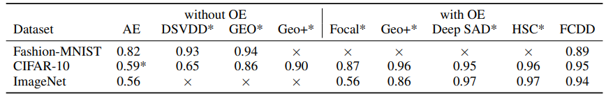
3.1.1 Quantitative results. FCDD, despite using a restricted FCN architecture to improve explainability, achieves a performance that is close to state-of-the-art methods and outperforms autoencoders, which yield a detection performance close to random on more complex datasets.
3.1.2 Qualitative results.
For a Fashion-MNIST model trained on the nominal class “trousers,” the heatmaps show that FCDD correctly highlights horizontal elements as being anomalous, which makes sense since trousers are vertically aligned.

For an ImageNet model trained on the nominal class “acorns.” Colors seem to be fairly relevant features with green and brown areas tending to be seen as more nominal, and other colors being deemed anomalous, for example the red barn or the white snow. Nonetheless, the method also seems capable of using more semantic features, for example it recognizes the green caterpillar as being anomalous and it distinguishes the acorn to be nominal despite being against a red background.

Below shows heatmaps for CIFAR-10 models with varying amount of OE, all trained on the nominal class “airplane.” As the number of OE samples increases, FCDD tends to concentrate the explanations more on the primary object in the image, i.e. the bird, ship, and truck.

3.2 Explaining Defects in Manufacturing
MVTec-AD. This datasets offers annotated ground-truth anomaly segmentation maps for testing, thus allowing a quantitative evaluation of model explanations. MVTec-AD contains 15 object classes of high-resolution RGB images with up to 1024×1024 pixels, where anomalous test samples are further categorized in up to 8 defect types, depending on the class. Network is based on a VGG11 network pre-trained on ImageNet, where the first ten layers were frozen, followed by additional fully convolutional layers that were learnable.
3.2.2 Synthetic Anomalies
OE with a natural image dataset like ImageNet is not informative for MVTec-AD since anomalies here are subtle defects of the nominal class, rather than being out of class. For this reason, synthetic anomalies is generated using a sort of “confetti noise,” a simple noise model that inserts colored blobs into images and reflects the local nature of anomalies.

3.2.3 Semi-Supervised FCDD
A major advantage of FCDD in comparison to reconstruction-based methods is that it can be readily used in a semi-supervised AD setting. To see the effect of having even only a few labeled anomalies and their corresponding ground-truth anomaly maps available for training, each MVTec-AD class is picked for just one true anomalous sample per defect type at random and add it to the training set. This results in only 3–8 anomalous training samples.
Pixel-wise objective function:
$$ \min_{\mathcal{W}} \frac{1}{n}\sum^{n}_{i=1}(\frac{1}{m}\sum^{m}_{j=1}(1-Y_j)A'(X_{i})_j) - \log(1-\exp(-\frac{1}{m}\sum^{m}_{j=1}A'(X_{i})_{j})) $$
Let \(X_1, \ldots , X_n\) again denote a batch of inputs with corresponding ground-truth heatmaps \(Y_1, \ldots , Y_n\), each having \(m = h \cdot w \)number of pixels. Let A(X) also again denote the corresponding output anomaly heatmap of \(X\).
3.2.4 Qualitative Results.
FCDD outperforms its competitors in the unsupervised setting and sets a new state of the art of 0.92 pixel-wise mean AUC. In the semi-supervised setting—using only one anomalous sample with corresponding anomaly map per defect class— the explanation performance improves further to 0.96 pixel-wise mean AUC. FCDD also has the most consistent performance across classes.

3.2.5 The Clever Hans Effect
The “Clever Hans” effect means that memory of the horse Hans, who could correctly answer math problems by reading its master. Roughly one fifth of all horse images in PASCAL VOC (Everingham et al., 2010) contain a watermark in the lower left corner. Lapuschkin et al. (2016; 2019) showed that a classifier recognizes this as the relevant class pattern and fails if the watermark is removed. This experiment is adapted to one-class classification by swapping our standard setup and train FCDD so that the “horse” class is anomalous and use ImageNet as nominal samples.
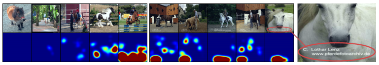
Center block shows that a one-class model is indeed also vulnerable to learning a characterization based on spurious features: the watermarks in the lower left corner which have high scores whereas other regions have low scores. The model yields high scores for bars, grids, and fences in left block. This is due to many images in the dataset containing horses jumping over bars or being in fenced areas. In both cases, the horse features themselves do not attain the highest scores because the model has no way of knowing that the spurious features, while providing good discriminative power at training time, would not be desirable upon deployment/test time. In contrast to traditional black-box models, however, transparent detectors like FCDD enable a practitioner to recognize and remedy (e.g. by cleaning or extending the training data) such behavior or other undesirable phenomena (e.g. to avoid unfair social bias).
4. Conclusion
FCDD performs well and is adaptable to both semantic detection tasks and more subtle defect detection tasks. Finally, directly tying an explanation to the anomaly score should make FCDD less vulnerable to attacks (Anders et al., 2020) in contrast to a posteriori explanation methods.


댓글